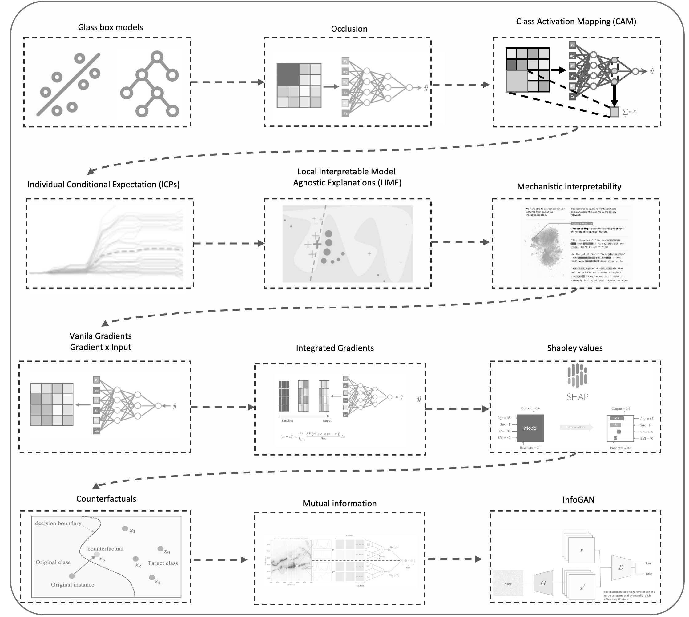
LIME explains a prediction by replacing the behaviour of a complex black box model with a
locally interpretable surrogate model. It is local in the sense that explanations are provided
on a per instance basis, and model agnostic since it can be applied to any model. Intuitively,
this method generates an artificial dataset by perturbing the instance in question. The idea is
simple: although the global structure of the decision boundary might be complex, locally the
boundary can often be approximated by a simpler (possibly linear) boundary. A model of this type
has readily interpretable weights. LIME is one of the few methods that can be applied across
data modalities.
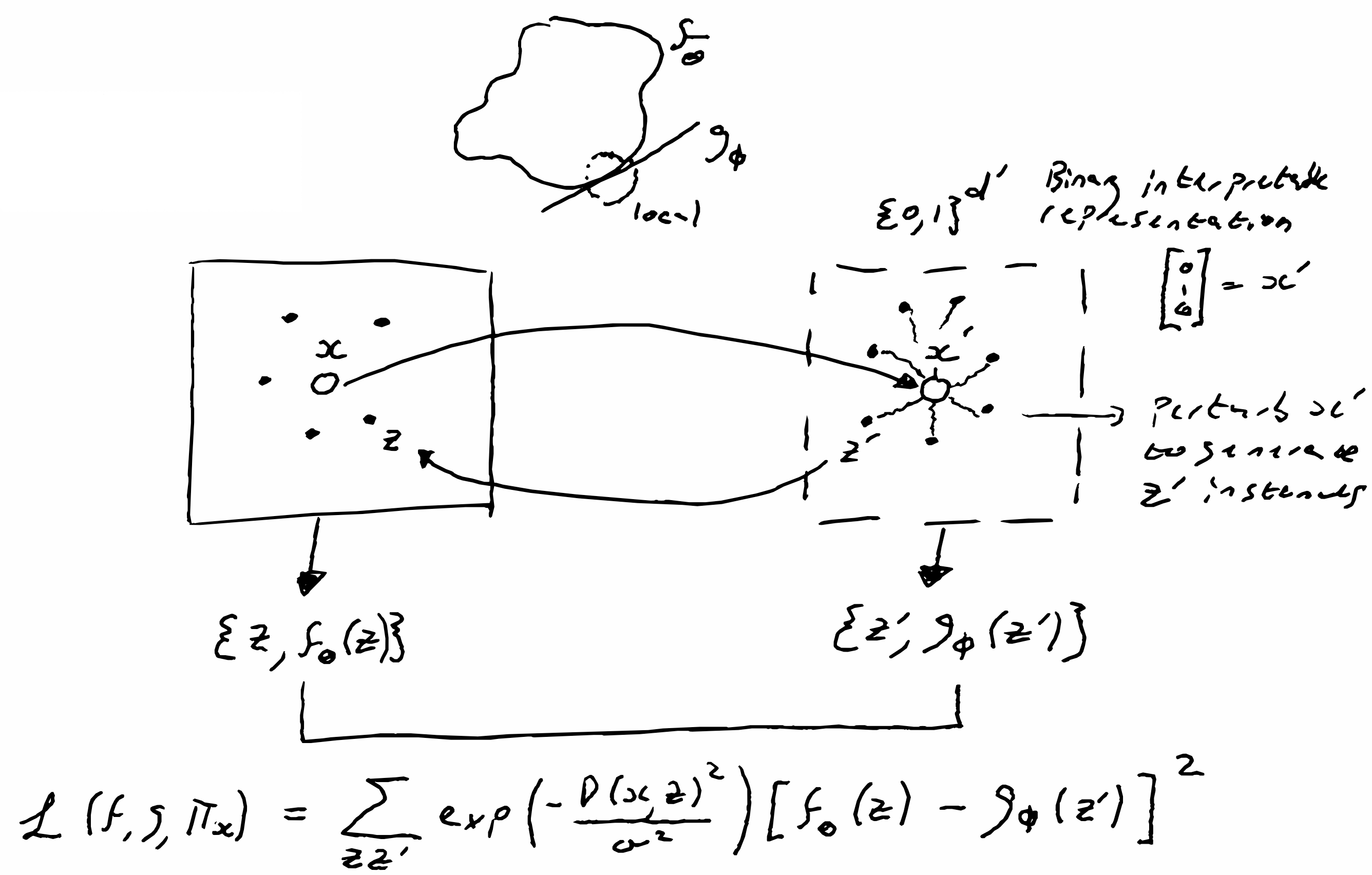
Procedure: Take a single data instance $x \in X$ that you want
to explain and transform it into an interpretable domain $x \to x^\prime$. Here $x^\prime \in
\{0,1\}^{d^\prime}$ is a binary vector, where the interpretable quanta are either present or
missing (the idea of missingness is central to XAI methods). Obtain a binary dataset
$\{z^\prime\}$ by randomly sampling from $\{0,1\}^{d^\prime}$. This sample is then transformed
back into the original data representation to give $\{z\}$. Act on the sample with the black box
model $f_\theta | z\to y$ to generate a labeled dataset $\{z,f_\theta(z)\}$. Then search for an
interpretable model $g \in G$ that acts on the interpretable domain $\{0,1\}^{d^\prime}$, such
that the local fidelity between the surrogate simple model is close to that of the actual model
operating in the original domain. The highly flexible training objective is given by
$$
\xi(x)=\underset{g \in G}{\operatorname{argmin}} ~\mathcal{L}\left(f, g, \pi_x\right)+\Omega(g).
$$
Here the fidelity is controlled by some loss function $\mathcal{L}$ that is made local by
incorporating a proximity measure $\pi_x(z)$, while $\Omega(g)$ penalizes model complexity and
is often human controlled. A concrete example of the loss function could be the squared loss
$$
\mathcal{L}\left(f, g, \pi_x\right)=\sum_{z, z^{\prime} \in \mathcal{Z}} \underbrace{\exp
\left(-\frac{D(x,
z)^2}{\sigma^2}\right)}_{\pi_x(z)}\left[f_\theta(z)-g_\phi\left(z^{\prime}\right)\right]^2,
$$
where the proximity measure $\pi_x(z)$ is an exponential kernel that places more weight on data that is similar to the point in question, i.e., only small perturbations and $D$
is some distance function (e.g., cosine distance for text, L2 distance for images). Note that
this is critical since the random sampling is done in an uncontrolled manner.
Although LIME is applicable to every model, it suffers from a few drawbacks. 1) The choice of
observable representation impacts the quality of the explanation. 2) The complexity of the
surrogate model (number of parameters $k=|\phi|$) is a hyperparameter that has to be tuned and
symbolizes the tension between fidelity and explainability. 3) The width $\sigma$ of the
proximity measure is another hyperparameter and possibly the weakest feature of LIME since for
complex points the size can flip the explanation. 4) Sampling from the binary representation is
done with a flat distribution (ignoring feature dependence) and could therefore lead to
perturbed datasets that do not faithfully represent the actual dataset, thus leading to poor
decision boundaries. 5) Decision boundaries might not be manifolds and therefore not locally
represented by a simple model.
The LIME quanta for images are superpixels, which are generated by standard algorithms that
partition the image into a "jigsaw" of patches that have similar visual qualities. For words,
LIME uses a bag of words for its quanta, while for tabular data, it is not necessary to
transport instances into interpretable representations; one can simply perturb each feature
according to the distribution of values for said feature.