DeepMoveSeek: Chain-of-Thought Reasoning as Semantic Tree Search

DeepMoveSeek is an exploratory research project on whether a Large Language Model (LLM) can support chess decision-making by producing structured chain-of-thought style reasoning that helps guide search over candidate lines of play. Rather than treating language as a purely post-hoc interface, the project investigates whether natural-language reasoning can play a more direct role inside a decision pipeline for complex sequential problems.

The core idea is not to claim that language fully replaces established chess search methods such as Monte Carlo Tree Search or classical engine search, but to study whether language can provide a useful semantic planning layer: proposing hypotheses, comparing alternatives, highlighting critical positional features, and helping prune unpromising continuations. In this sense, the project sits at the intersection of reinforcement learning, reasoning models, and interpretable decision support.

A major motivation is that conventional chess AI is extremely strong, but often difficult to connect to natural-language explanations that are faithful to the actual decision process. DeepMoveSeek explores whether this gap can be narrowed by training a model whose intermediate reasoning is more tightly coupled to move selection. The goal is not to claim guaranteed interpretability, but to investigate a system in which reasoning traces are more closely linked to downstream actions than in standard post-hoc explanation pipelines.

The project is also motivated by the fact that human chess annotations are often limited: they can be sparse, stylistically inconsistent, and not always tightly aligned with the objectively strongest move. Chess, however, offers an unusually valuable research setting because strong external engines provide a reliable source of evaluation and supervision. DeepMoveSeek therefore uses a deterministic truth oracle in the form of high-quality engine analysis to study how language-based reasoning can be shaped by objective feedback.

Methodologically, the project draws inspiration from recent advances in reasoning-oriented language-model training, including systems that combine supervised warm-starts, reinforcement learning, and distillation. The contribution here is not the invention of those ingredients themselves, but their adaptation to a chess setting in which reasoning quality can be evaluated against a strong external engine. This makes chess a useful testbed for studying when language-based reasoning is genuinely helpful, when it collapses into plausible-but-unfaithful narration, and how reward design influences that trade-off.

A typical training pipeline begins with a small corpus of engine-annotated examples to bootstrap coherent reasoning traces. This is followed by a reinforcement-learning phase in which candidate lines of reasoning are evaluated according to the quality of the moves they produce under engine-based feedback. A final filtering or distillation stage can then be used to retain the most useful traces and compress them into a smaller model for deployment. An important part of the research is empirical: designing experiments that test whether the language traces improve move quality, search efficiency, or explanation faithfulness in a measurable way.

More broadly, DeepMoveSeek is intended as a controlled research prototype for studying language-guided decision making. Chess provides a clean domain with strong evaluation tools, making it possible to test ideas about reasoning, supervision, and interpretability under conditions where outcomes can be measured precisely. While the project is domain-specific, the longer-term interest is whether similar training principles could help build AI systems whose reasoning is not merely fluent, but more usefully connected to the decisions they make.

Multimodal Chess: CLIP-Style Contrastive Alignment for Position and Language

A recurring obstacle in chess AI is that the knowledge encoded in strong analytic engines (precise, numerical, positional) and the knowledge encoded in human expert commentary (conceptual, strategic, verbal) exist in entirely separate representational spaces with no principled bridge between them. This project constructs that bridge by training a self-supervised multimodal model, inspired by contrastive learning frameworks such as CLIP, on a curated dataset of (position, text) pairs. The result is a joint embedding space in which strategically similar concepts across both modalities are geometrically close, enabling retrieval that is grounded in meaning rather than surface-level pattern matching.

Initial representations are generated independently for each modality. Deep positional embeddings are extracted using the pre-trained LCZero engine, whose internal activations encode rich strategic and tactical structure accumulated through self-play. Semantic text embeddings are produced by pre-trained sentence transformer models trained to capture the meaning of natural language at the level of full sentences and paragraphs. The contrastive training objective then learns a transformation that pulls together embeddings of a position and its corresponding expert analysis while pushing apart unrelated pairs. This alignment procedure is the core innovation: it does not require explicit labels beyond the pairing itself, making it scalable to large corpora of engine-annotated games and their associated commentary.

The aligned space is then exploited by a Retrieval-Augmented Generation (RAG) system. When a new chess position is provided, its embedding is projected into the joint space and a nearest neighbor search (using vector databases such as FAISS, Milvus, or Pinecone) identifies the expert text snippets whose embeddings are most semantically proximate. Crucially, proximity here reflects deep strategic and conceptual relatedness learned during contrastive training, not superficial board similarity. Different retrieval strategies operating within this space are compared to optimize for context that is maximally useful for explanation generation.

The retrieved context and input position are then passed to an instruction-tuned LLM via carefully engineered prompts that include the position in FEN notation, a target ELO level, the retrieved text snippets, and explicit instructions for the desired output format. This ELO-conditioned generation allows the system to tailor the depth and vocabulary of its explanations to the level of the user, producing feedback that is strategically accurate for a grandmaster and pedagogically accessible for a club player. Parameter-Efficient Fine-Tuning (PEFT) is explored where needed to sharpen this ELO-specific tailoring without full model retraining.

The broader interest of this work lies in demonstrating that contrastive multimodal alignment can serve as a general mechanism for grounding language models in structured, non-linguistic domains. Chess provides an unusually clean testbed: the ground truth is unambiguous (engine evaluations), the modality gap between board states and natural language is large, and the diversity of available expert commentary is rich. A retrieval system that successfully bridges this gap offers a concrete proof of concept for analogous problems in scientific domains where formal representations and natural language descriptions coexist but remain poorly integrated.

Explainable Artificial Intelligence

One of the major problems in the field of deep learning is model opacity. This was a natural consequence of ML being raised and nurtured in an industrial environment, where performance superseded understanding. The deep learning revolution further exacerbated the problem of model capacity, where it was found that instead of relying on the carefully hand-crafted features of scientists, one could do away with Newton by simply adding more layers to the network. Furthermore, the fact that complexity is often correlated with higher performance leads to black boxes, representing an unrevealed tension between the values of the scientific method and the design mode of machine learning models. The opacity of deep learning models can be reduced via the application of various gradient attribution methods. These methods can for example highlight the discriminant region of a network trained on a binary classification task. To validate our application of these techniques before aiming them at a serious research question, we applied them to a toy problem of identifying sunspots from pores. In this case, we know that the distinguishing feature is the presence of a penumbra (the intermediate grey region between the dark center and light surroundings). We discuss two methods here, the first requires measuring the sensitivity of the output with regards to the final convolutional layers in a CNN, while the second works at the level of the input directly via the application of a method from competitive game theory.

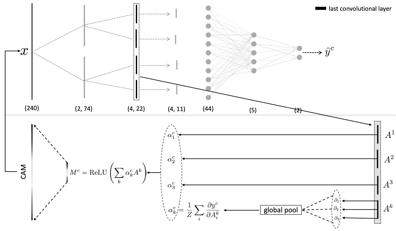
The first method called Gradient-weighted Class Activation Mapping (Grad-CAM) is derived from a simpler implementation called CAM. The idea is that the most important spatial representation of the input resides in the final convolutional layer before the dense layers. The spatial information does not survive a pass through the dense layers since they are fully connected (mixed). The authors of CAM noticed that if they fed the final convolutional layer directly into a softmax, then the weights of the single dense layer can be used to directly evaluate the importance of each pattern picked up by the final maps. A heatmap/salience map of the discriminant region can then be obtained by projecting back a weighted linear sum of the final feature maps, where the weights correspond to the weights of the softmax layer. This setup represents a significant architecture constraint, namely that you have to go straight from the convolutional layers into a softmax.

Grad-CAM also derives a heatmap from a linear sum of the final feature maps in the CNN, however, the weights are derived as the sensitivity of the output prediction with respect to the final feature maps. As can be seen in the above 1D illustration, the heatmap is given by $$ M = \text{ReLU}\left(\sum_k \alpha_k A^k\right) $$ where the weights $\alpha_k$ for each on the final convolutional feature maps $A^k$ are given by the pooled/average gradient of the output with respect to the pixels in each feature map $$ \alpha^c_k = \frac{1}{Z}\sum_i\frac{\partial y^c}{\partial A^k_i}. $$ Notice that the output is wrapped in a ReLU activation function so that only positive gradients are considered, i.e., explanations that increase the prediction and therefore correspond to the positive class. In this way, one can judge the importance of a particular pattern from the input by simply monitoring the sensitivity of the output to first order with respect to the final feature maps. This gradient trick represents a significant improvement over CAM, and elevates the method to the class of gradient attribution methods, where any convolutional architecture can be used. One important thing to note is that the resolution of the explanation is at the same resolution as the final feature maps, which by convention tends to shrink as you move to deeper layers in the network. This requires the final saliency map to be extrapolated back to the original dimensionality. It also means that although we have got rid of many restraints, the quality of the explanation is still tied to, and is dependent on, the model's final architecture.

It would be desirable to have a model-agnostic method that does not rely on the special units of a CNN. Such a method is called Expected-Gradients (EG) and it borrows ideas from competitive game theory. It turns out that there exists a one-to-one mapping between the proper and fair distribution of monetary rewards to individuals based on their contribution and the distribution of a model's predictions amongst its inputs. The value that determines a player's contribution to getting a final reward is called the Shapley value $$ \phi_{\lambda}(\mathcal{F}_\Theta)=\sum_{S \subset N} \frac{(s-1) !(n-\mathrm{s}) !}{n !}[\mathcal{F}_\Theta(S)-\mathcal{F}_\Theta(S-\lambda)], $$ where $\mathcal{F}_\Theta$ is some black box model or game (in this case it can be thought of as the market), and $\lambda$ are the individual player of the game. This formula says that a player's worth is the average difference between what would have been earned with and without said player over all possible subsets/coalitions of players. The need to traverse all subsets is due to the possible non-linear dependencies between performance and coalitions.
We can replace the market $\mathcal{F}_\Theta$ with our black box ML model. The people $\lambda$ become individual pixels of our images, and the monetary reward can be mapped to the model's output prediction in our binary classification pore/sunspot task. In other words, instead of fairly distributing rewards, we use the Shapley value formalism to fairly distribute the model's prediction, i.e., finding out which parts of the input is most responsible for said prediction.

The only complication is that it is not entirely clear how to implement the idea of a subset in the case of a deep learning model. NNs required information to continually flow through all their channels. One workaround is to feed in a baseline for missingness, such that the expectation value of the baseline has a net zero effect on the final model output. Selecting a tensor of zeros is a bad idea since zeros might be critical in images as they function as borders and outlines. Another idea for missingness is to feed the network Gaussian noise. Although this is an improvement, it comes with the assumption that each pixel is independent of one another. This disregard for the possible wealth of interdependence between pixels will result in an unfair estimation of contribution. To mitigate this, EG uses the dataset itself as a baseline. The deep learning equivalence of the classically Shapley value formalism is given by $$ \begin{align} \phi_\lambda|_\text{EG} &=\int_{x^{\prime}}\Bigl(\left(x_\lambda-x_\lambda^{\prime}\right) \times \\ & \times \int_{\alpha=0}^{1} \frac{\delta \mathcal{F}_\Theta \left(x^{\prime}+\alpha\left(x-x^{\prime}\right)\right)}{\delta x_\lambda} d \alpha\Bigr) p_{D}\left(x^{\prime}\right) d x^{\prime} \\ &\simeq\underset{x^{\prime} \sim D, \alpha \sim U(0,1)}{\mathbb{E}}\left[\left(x_\lambda-x_\lambda^{\prime}\right) \frac{\delta \mathcal{F}_\Theta\left(x^{\prime}+\alpha \times\left(x-x^{\prime}\right)\right)}{\delta x_\lambda}\right], \end{align} $$ where $x$ is the target image in question. Here, we interpolate the image from a random baseline image $x^\prime$ into the target image in question by progressing $\alpha = 0 \to 1$. During the translation to the target image, the target features emerge and we monitor the accumulated gradient of each pixel with respect to the model's output prediction. This is done for multiple baselines such that on average, the gradients cancel after the expectation, and we have a fair evaluation of how important each pixel is for the prediction. Notice that in order to form pseudo subsets we have to pick up an additional integration factor.

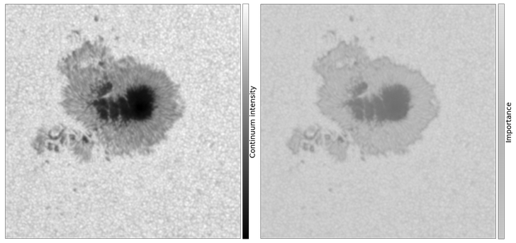
We note that working directly at the resolution of the input data often results in non-smooth saliency maps. EG is therefore often used as a differential prior during training, and a smoothness condition requiring small changes between proximal pixels is invoked. The results of Grad-CAM and Expected gradients were extremely complementary, with the above image showing that indeed the network pooled its attention (orange colors) into the discriminant structure, namely the penumbra. This is exactly what a human would base their decisions on when trying to classify these images.

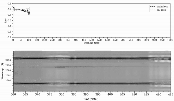The animation above illustrates how the model’s attention progressively converges on an important feature in the spectrogram of an IRIS observation during training. The model was trained for solar flare prediction. The top panel displays the training loss; as the model becomes more skillful, its attention narrows and highlights a critical pre-flare spectral signature in the IRIS spectrogram.

Reinforcement Learning for Non-LTE Radiative Transfer

We present a novel reinforcement learning (RL) approach for solving the classical 2-level atom non-LTE radiative transfer problem by framing it as a control task. An RL agent learns a depth-dependent source function $S(\tau)$ that self-consistently satisfies the equation of statistical equilibrium (SE). The agent's policy is optimized entirely via reward-based interactions with a radiative transfer engine, without explicit knowledge of the ground truth.

This method bypasses the need for constructing approximate lambda operators ($\Lambda^*$) common in accelerated iterative schemes. It requires no extensive precomputed labeled datasets to extract a supervisory signal, and avoids backpropagating gradients through the complex RT solver itself. The central insight is that statistical equilibrium can be enforced as a reward signal rather than a hard analytical constraint, turning what is traditionally a fixed-point iteration problem into a sequential decision-making task.

We also show through experiment that a simple feedforward neural network trained greedily cannot solve for SE, possibly due to the moving target nature of the problem (the optimal source function at each depth depends on the source function everywhere else), creating a non-stationary optimization landscape that confounds greedy supervised approaches. The RL framework naturally handles this non-stationarity through its policy gradient updates, which account for the long-range dependencies encoded in the discounted return.

The $\Lambda^*$-Free method offers potential advantages for complex scenarios (atmospheres with enhanced velocity fields, multi-dimensional geometries, or complex microphysics) where $\Lambda^*$ construction or solver differentiability is challenging. Additionally, the agent can be incentivized to find more efficient policies by manipulating the discount factor $\gamma$, leading to a reprioritization of immediate rewards and potentially more computationally economical convergence paths.

If demonstrated to generalize past its training data, this RL framework could serve as an alternative or accelerated formalism to achieve SE. To the best of our knowledge, this study represents the first application of reinforcement learning in solar physics that directly solves for a fundamental physical constraint.

Calculating Mutual Information by Sampling Raw Data

We applied a deep learning framework to calculate the information shared between two random variables of any dimensionality without discretizing the original data via a vector quantization. The quantity we were after is one of the cornerstones of information theory called Mutual Information (MI). It characterizes the total degree of dependence between two random variables. In technical terms, the MI represents the decrease in entropy of random variable $X$ after observing random variable $Y$, where entropy (specifically Shannon entropy $S(X)\coloneqq\mathbb{E}[-\log p(X)]$) is a functional that takes in a probability distribution and outputs a real value that represents the average number of binary questions required to determine the value of said random variable. Intuitively, entropy characterizes how distributed or clumpy the probability mass is over the state space, and MI tells us how much information we can extract from $X$ given $Y$. Unlike the classical Pearson correlation coefficient, MI captures the total (both linear and nonlinear) degree of dependence by measuring the discrepancy (by means of the KL-divergence) between the baseline uncorrelated state, naturally given by the product of the marginals, and the joint probability distribution. The discrete form of MI is given by $$ MI(X, Y) \coloneqq \sum_{x\in X}\sum_{y\in Y} p(x,y) \log \left[\frac{p(x,y)}{p(x)p(y)}\right]. $$ One can create a numerical foothold and turn the above calculation into a variational optimization problem by recalling Donsker and Varadhan's dual representation of the KL-divergence $$ D_{\mathrm{KL}}(p \| q)=\sup _{T: \Omega \rightarrow \mathbb{R}}\left\{\mathbb{E}_p[T]-\log \left(\mathbb{E}_q\left[e^T\right]\right)\right\}. $$ The idea here is simple. One can measure the difference between two objects by measuring the difference between their outputs when processed through the same function $T$. This function takes in an object of some undisclosed dimension $\Omega$ and reduces it to a scalar value in $\mathbb{R}$. What remains is the careful construction of this functional. With all variational problems, we start with an educated guess and slowly transverse the space of possibilities in a controlled manner until we hit upon something close to the supremum allowing us to achieve a tight lower bound for the estimate of the MI. We can parameterize the function $T$ with a neural network $T_\theta$ $$ M I(X ; Y)_n \geqslant \sup _{\theta \in \Theta}\left\{\mathbb{E}_{P_n}\left[T_\theta\right]-\log \left(\mathbb{E}_{P_n^{\dagger}}\left[e^{T_\theta}\right]\right)\right\}, $$ and then use gradient descent to traverse the space of all possible functions quickly. For notational convenience, the joint probability is represented by $P$, while the product of the marginals is given by $P^\dagger$. A simple architectural choice for the network is an encoder that can compress the input into a scalar-valued output, i.e., something that can induce the desired transformation $\Omega\to\mathbb{R}$. Furthermore, the general high expressibility of neural networks guarantees a tight lower bound. It is also important to note that we can only ever underestimate the MI with this representation. The particular architecture and training schedule that realizes the dual representation is called a Mutual Information Neural Estimator [cached]or MINE-network

The image shows a practical distillation of the above mathematical abstractions. The insert on the left is taken by one of NASAs small explorer satellites IRIS, whose mission is to provide insights into the mechanism leading to the coronal heating problem (a remarkably unintuitive phenomenon where the Sun's outer atmosphere, its corona, is orders of magnitude warmer than its inner atmosphere). The satellite generates a small field-of-view image of the Sun as well as spectra from different atomic ions. Each pixel in the above image contains multiple spectra recorded simultaneously, such that each pixel serves as a sample point for multiple random variables. The random variables in our case are extended line profiles living in $\mathbb{R}^{240}$, whose shapes are forged via the joint action of radiative transfer and basic atomic theory. Each line shape encodes to some extent the physical attributes of the solar atmosphere within a particular temperature range. We can apply the MINE-network to two spectral lines Mg II and C II and derive their MI. The network itself is relatively simple being composed of a series of simple encoders that force the spectra down to scalar values. The fancy footwork can be found in how the data is sampled. The top channel (above the dotted line) takes Mg II, and C II spectra from the same pixel at the same moment in time, and therefore samples from the joint probability distribution P. The bottom channel on the other hand takes the spectra from two different pixels, therefore, sampling from the product of the marginals $P^\dagger$ and providing a baseline uncorrelated state. This baseline is made more accurate if the sampling is also random across the time domain. The encoder then consumes the spectra and finds a latent variable representation in $z$. The new representation is then concatenated and further reduced to a scalar value by a final encoder. It is important to keep in mind that the encoder complex shares parameters for both the upper and lower sampling channels. The network is then charged with the task of trying to separate the two scalar value outputs from both channels using any means possible. Since the lower channel provides by definition the baseline uncorrelated state, the only way the encoder complex can distinguish between the two channels is to learn all possible correlations that exist between the lines drawn from the same pixel. The further apart the network can pull the scalar values, the more information the two variables/lines share. These scalar values can then be fed into the above dual formula resulting in the MI. We compared the results for an ensemble of different spectral line-pairs as well as against a discrete method and found that both methods produce the same results and that the lines that share most information have similar atomic physics and formation heights. The information quantity between almost all lines are also enhanced in regions of increased energy deposition, meaning massive events such as solar flares open up the communication channels at different scale heights. The confirmation of the results from multiple sources proves that the MINE-network provides a hands-free way of calculating a critical information-theoretic quantity between any two random variables of any dimensionality.

Vector Quantization to Analyze Millions of High Energy Spectra

The k-means algorithm is one of the most successful ML algorithms of all time. It is a simple and elegant algorithm that can be used to cluster data points of any dimensionality into groups. In technical terms, it is an example of an unsupervised learning method that can be used to find the optimal number of clusters in a dataset by modeling the underlying density via a vector quantization. At its heart, k-means can be thought of as a type of generalized binning, where normally we would impose a binning on scalar values, k-means allows us to bin together abstract vectorial objects such as shapes. If you are willing to relinquish high-frequency small variations, then k-means can offer you a foot into the realm of statistical analysis, as well as reduce model complexity for upstream tasks. The algorithm introduces $n$-centroids (the models only hyperparameter) and then iterates between two steps, an assignment step $$ S_i^{(t)}=\left\{x_p:\left\|x_p-\mu_i^{(t)}\right\|^2 \leq\left\|x_p-\mu_j^{(t)}\right\|^2 \forall j, 1 \leq j \leq k\right\}, $$ where points are assigned to their closest centroids $\mu_i$, and an update step $$ \mu^{t+1}_i = \sum_{xj\in S^{(t)}_i}x_j / |S^{(t)}_i|, $$ where the centroids are updated to the mean of the points assigned to them. Here, $t$ is the discretized time variable keeping track of the iterations, while $S=\{S_i\}$ is the imposed partitioning of the dataset into $k$ groups. The algorithm converges when the centroids stop moving. The algorithm is simple and elegant, but it has a few drawbacks. Firstly, it is not guaranteed to converge to the global optimum, and secondly, it is not guaranteed to converge to the same solution every time. To help alleviate this problem the algorithm is often run multiple times with different initializations, and the best solution is chosen. It is also an example of a hard assignment algorithm, meaning that each point is assigned to a single cluster. This can be problematic if the data is not well separated. In such a case one should rather use a Gaussian mixture model which initiates several Gaussian distributions and then performs a soft assignment after iterating through a chain of optimization steps guided by the Expected Maximization algorithm. Finally, it is often very difficult to select the optimal number of clusters, and this is often done by trial and error and is not even guaranteed to have a definite answer. We used the algorithm to provide a tractable blueprint of all possible Mg II spectral shapes generated during a solar flare. This algorithm allowed us to automate the analysis of massive amounts of data by highlighting regions of the image where a particular emission was present. We found unique spectra with blue-shifted central reversals at the edge of fast-moving flare ribbons that coincided with strong X-ray signatures. We also discovered a universal flaring profile whose physical origin was later explained. Our solution for selecting the optimal number of centroids involves a loss function with three components, two of which require an additional but complementary dataset that is somehow co-spatial and temporal. The choice for the optimal number of groups can theoretically be automated by 1) Finding the elbow in the variance as a function of group number (i.e., change between fast to slow gains with additional centroids) 2) Require some spatial coherence by enforcing some differential prior to promote continuity between neighboring pixels and their assignments, and 3) Maximize the MI between the assigned groups and the co-spatial dataset. A generic loss function can be constructed by appropriately weighing each of these components.

Transformers for multivariate time Series Analysis

Analogous to how kernels in CNNs update themselves to identify important patterns and features of the input, transformers dynamically adapt the constellation of vectors called an embedding, whose cosine distance shuttles information from an abstract space containing words into a machine consumable vector representation. The quality of this embedding directly determines how accurately the information is grafted into the algorithm. Transformers modify embeddings in several ways. In natural language processing (NLP), the zeroth order approximation is to first transport the words into vectors using a one-hot encoding scheme. This assumes no prior connection between the words since the cosine distance between all vectors in an orthonormal configuration is equal. The orthonormality is then broken using an algorithm like word2vec, which collects frequency information about the occurrence of words in the same sentence over a corpus of text. The end result of this first-order correction is that words that have similar meanings are shifted closer together. An important thing to notice here is that this correction is done globally, and therefore lacks contextual nuance since it is a massive average over the entire textual corpus. Since transformers are invariant under permutations of the input, a second-order correction is added in the form of positional embedding, which respects the influence that order has over the meaning of a sentence. The final correction is what elevates transformers above other sequence-type models, and that is a fine-scale dynamic third-order correction that fuses context into the embeddings via the use of the self-attention mechanism. Instead of applying transformers to problems in NLP, we are using their powerful representational abilities to analyze multi-variable time sequences (mvts). In this framework, several things have to be adjusted. Firstly, an algorithm like word2vec need not be used since the distance between feature vectors $x_t$ are already meaningful. Here $x_t$ is a single slice of the input mvts as seen in the above image, representing the state of all variables frozen at time $t$. Next, instead of using the normal layerwise normalization scheme for NLP, it is advisable to use batch normalization which is better at handling outliers, as well as constructed learned positional embeddings over the standard sinusoidal variant. This transformer encoder as seen in the above image takes an input of size (batch, sequence_length, feature_dim) and enriches the embedding by cycling it through what is called a multi-headed self-attention unit. The data $X$ is first made sensitive to order by infusing the constellation of vectors with a positional embedding resulting in $\tilde{X}$. The embedding is then forced into the model dimension $U$ of shape (batch, sequence_length, model_dim) before it is linearly projected into three different representations via the use of matrices $Q,K$, and $V$ with learnable weights. These matrices allow each input feature vector $x_t$ to interact with one another, discover which vectors are contextually tied together, and then use those vector subsets to inform an updated embedding based on the context of the surrounding information. The reason for the three representations is that the engine that powers this reshuffling of the embedded vectors is the simple scaled dot product. With such a simple mechanism, three representations are the minimum number required for the contextual embedding to be unrestrained, i.e., any vector can migrate in any direction. The embedding is updated as follows: The scaled dot product is taken between all the vectors of representation $i$ and $j$ of the input, resulting in a probability distribution. This distribution is used to form a weighted sum of all the vectors in subspace $k$, allowing the vector in question to be updated, and therefore changing its cosine relation with the entire constellation. These steps of dot product, weight, and update can be seen as imbuing the constellations with an attractive force. If we have a single representation $i=j=k$, then the procedure under the simple action of the scaled dot product will result in an attractive force between all proximal vectors, which unless you believe the data should be massively binned due to a gross amount of redundancy, then such a transformation cannot be beneficent. If instead, you use two representations, then vectors that are contextually dependent will cluster together, which again is not useful, since it implies that things that are contextually bound can be interpreted as the same object. Finally, having three representations allows the identification of context via the scaled-dot product of the first two, while the new embedding can be updated in any direction via the sourcing of vector values of the third representation. In summary, a space is made in a transformer, where driven by the particular objective function of the upstream task, the local sequence of vectors can communicate with one another, and freely (without restraint) rearrange themselves to dynamically infuse context into their embedding. The presence of skip connections is to stabilize the gradients, resulting in slow updates to the embedding. This entire process can be massively parallelized via the use of matrix operations. The attention head described above is carried out in parallel with several (usually eight) different heads with separate $Q, K$ and $V$ matrices. The entire system is cycled several times resulting in a massively aggregated final embedding $Z$ which can then be used for any upstream task such as classification, regression, or decoding. The point of the cycles is to amplify the contextual embedding, while the multi-headed aspect appears to be linked (in my opinion) to the fact that context, like an explanation in XAI, is an ill-defined metric and all such metrics cannot be parameterized mathematically and subjected to optimization via gradient descent. When this is the case the Monte Carlo method of large statistically averaged ensembles appears to be the best alternative. I am using a transformer encoder now to evaluate the capacity to predict flares based on mvts from the Solar Dynamic Observatory. I am also using the attention matrices for the analysis of variable dependence, as well as modifying the multi-headed system using ideas from information theory.

t-Distributed Stochastic Neighbor Embedding

We often want to reduce the dimensionality of our data, while preserving its fundamental geometric and topological structure. One motivation is to preserve only the most relevant aspects of the data for some upstream more complicated tasks, thus leading to better model clarity and lower computational expense, as well as mitigating the curse of dimensionality, where data starts to crowd along the edges due to volume scaling rules. Another motivation is to visualize high-dimensional data in a 2D or 3D space. While techniques such as principal component analysis (PCA) serves the prior task, t-SNE is a non-linear dimensionality technique that allows one to flexibly preserve the geometry of high dimensional data in lower dimensional embeddings at any granularity. It accomplishes this as follows. First, the algorithm translates the point-wise distance matrix into a statistical distance matrix $D\to P$, by placing multidimensional Gaussians over each data point and measuring the overlap of the distributions between points. The Gaisians are then allowed to dynamically shrink or expand depending on a single controllable hyperparameter called the perplexity $2^{-S}$, where $S$ is the Shannon entropy. Setting the perplexity to a small value results in a small entropy and consequently Gaussian distributions that have tight variances. On the other hand, a large perplexity will act to broaden the Gausians. Note that in order for the perplexity to be met, each Gusian dynamically alters itself depending on the local density of the data, thus infusing t-SNE with a relative distance measure. This can be seen in the upper left image. The Gaussian centered over the point $x_i$ has to expand its variance to achieve the same entropy as the Gaussian centered over point $x_j$ which finds itself in a far denser region. The low-dimensional embedding is then initiated by guessing a random prior (right-hand insert in the above image) for the positions of the $N$ data points. In the same way as before, a statistical distance matrix $P^\dagger$ is constructed, this time via the use of student's-t distributions centered at each point to mitigate the crowding effect. The prior is then variationally improved by performing gradient descent on the KL-divergence $KL(P|P^\dagger)$. The idea of statistical distance along with perplexity allows t-SNE to either probe the local or global geometric structure of the data. For instance, a low perplexity would imply tight Gausians, and therefore each point would only be aware of its local neighborhood, thus leading to a local embedding. On the other hand, a high perplexity would imply broad Gausians and therefore allow each point to be aware of the entire dataset, thus leading to a global embedding.

Neural-ODEs

Normalizing flows allows us to transform a simple distribution into a more complex distribution via the change of variables formula (Tabak, Vanden-Eijnden, 2010). They are typically constructed via the composition of a string of invertible transformations, each of which is severely restricted in its form such that the calculation of the Jacobian determinant is computationally tractable. These restrictions can be relieved if one models the flow as a continuous time dynamic. In this framework, a neural network is used to model a vector field that transports the probability mass function into a new configuration along the field lines, resulting in a free-flow Jacobian (Chen et.al 2018). The problem reduces to an ordinary differential equation with initial conditions and can be solved using any black box ODE solver. To parley with ordinary NF models, the model depth is now determined by the density of the time grid. Typically one wants to approximate the density of some unknown distribution. This can be achieved by leveraging the symmetry of the configuration by simply flipping the integration limits. One samples from the real unknown distribution then maximizes the probability of the data after the flow under some base distribution that is easy to sample from and has a known density. Once this mapping is learned, then we can sample from the base distribution and “flesh out” the more complex unknown distribution. A point in training the system: It is computationally expensive to backpropagate through the ODE solver explicitly, so typically one uses the adjoint sensitivity method which turns the black box on itself to derive the loss functions dependence on the neural-ODEs parameters. This is done by solving another ODE with the same black box solver backward in time. The paradigm shift here is allowing the function responsible for the dynamics to be programable. Flows can be computationally optimized to form smoother trajectories (Finlay et.al 2020), made scalable using unbiased estimators for the likelihood (Grathwohl et.al 2018), as well as mitigate the topological conservative property of diffeomorphisms by introducing augmentations to the space on which the flows are learned (Dupont et.al 2019)(similar to the kernel trick for SVMs). An example of a Neural-ODE is shown below. In both cases, the neural network is used to model a vector field that transports the probability mass distribution from a simple 2-dimensional Gaussian base distribution to a more complex target distribution. One gains instructions on how to train the system by minimizing the KL-divergance between the target distribution and the flow distribution: $$\begin{aligned} \mathcal{L}(\boldsymbol{\theta}) & =D_{\mathrm{KL}}\left[p_x^*(\boldsymbol{x}) \| p_x(\boldsymbol{x} ; \phi)\right] \\ &\approx -\frac{1}{N}\sum_{n=1}^N \underbrace{\log p_u\left(T^{-1}(x_n;\phi)\right)}_{\substack{\text{maximize likelihood of flow}\\ \text{under the base distribution}}} + \underbrace{\log~\left|\det J_{T^{-1}}(x;\phi)\right|}_{\substack{\text{promote simpler transformations}\\ \text{that augment the space less}}}- \underbrace{S(p^*_x)}_{\substack{\text{entropy of target}\\ \text{distribution not used} \\ \text{in optimization}}}\end{aligned}$$ The target data is sampled and the likelihood of the resultant flow is maximized under the base distribution. The loss function is then given by the negative log likelihood of the data under the base distribution plus the log determinant of the Jacobian of the flow. The Jacobian determinant is used to promote simpler transformations that augment the space less. The entropy of the target distribution is not used in the optimization. After modeling the systems infintismal dynamics $\partial_t\boldsymbol{z}_t = g_\phi(\boldsymbol{z}_t, t)$ we extract the transfomraiton $T$ by integrating over time, resulting in the folowing ODE $$\underbrace{\left[\begin{array}{c} \mathbf{z}_0 \\ \log p(\boldsymbol{x})-\log p_{z_0}\left(\boldsymbol{z}_0\right) \end{array}\right]}_{\text {solutions }}=\underbrace{+\int_{t=t_1}^{t_0}\left[\begin{array}{c} g_\phi\left(t, \boldsymbol{z}_t\right) \\ -\operatorname{Tr}\left\{J_{g_\phi(t,)}\left(\boldsymbol{z}_t\right)\right\} \end{array}\right] d t}_{\text {dynamics }}, $$ which can be solved using the following initial conditions along with the PyTorch ODE solver $$ \quad \underbrace{\left[\begin{array}{c} \boldsymbol{z}_1 \\ \log p(\boldsymbol{x})-\log p\left(\boldsymbol{z}_1\right) \end{array}\right]=\left[\begin{array}{c} \boldsymbol{x} \\ 0\end{array}\right]}_{\text {initial values }}. $$

Our team is busy designing a computationally efficient continuous normalizing flow model using the adjoint sensitivity method to extract the full posterior distribution from non/LTE inversions of spectrophotometric signals taken by the swedish solar telescope. Results are pending.

CycleGAN / The coronal heating problem

The Coronal heating problem is one of the most perplexing problems in Solar physics. At the Sun’s visible surface, the temperature is a few thousand degrees Kelvin; however, as we move further away from our star's surface, the temperature rapidly increases by several orders of magnitude, characterizing the solar Corona, the Sun’s outer atmosphere. This unintuitive phenomenon has two proposed (not necessarily mutually exclusive) explanations. The first is that the Sun is a magnetohydrodynamic plasma, and as such, it is capable of supporting a large variety of wave-type oscillations that could possibly transport energy from deep below its surface up into its Corona. The other theory is that small magnetic reconnections between the upper canopy of magnetic loops are constantly sustaining the Coronal temperatures by converting magnetic energy into heat energy. The only problem is that we cannot directly observe these so-called nano-flares. As pointed out by Patrick Antolin, we can, however, indirectly observe nanoflares by looking for their byproducts. One such byproduct is the creation of thermal instabilities within the loops that can lead to catastrophic cooling and the condensation of denser cooler material that plummets back to the Sun’s surface. These dense, cool clumps of falling plasma are aptly named "coronal rain," and if one can somehow measure the amount of rain, then working backward it should be possible to reverse engineer the contribution of nanoflares to the coronal heating problem. Here is the catch… The instrument that observes the entire Sun has a broad bandwidth that lets in a hot component from the Si XI transition, which contaminates the images with diffuse hot coronal emission. On the other hand, NASA's IRIS satellite does not see the entire solar disk (only small patches); however, its passband is tight enough such that this unwanted stray light contamination is not present, making it easier to track cool, dense downflowing material. The

idea is to imbue the full disk images of SDO with IRIS quality. We, therefore, made use of a special generative adversarial network called a CycleGAN. In general, a generative model is trying to perform an interpolation between points on some latent space that the model develops. These methods try to find a latent space that is at least locally Euclidean so that we can do some vector calculus. There are many flavors of generative models such as VAEs, normalizing flows, and diffusion models, to name a few. A GAN is a type of generative model that borrows ideas from game theory. It is composed of two competing networks involved in a zero-sum game. The first network is called the generator $G$, and it takes in noise and generates an image $x^\prime$ belonging to a particular distribution or class. The second network called the discriminator $D$ then tries to discern whether this image is real $x$ or fake $x^\prime$. Both networks are in competition with one another where $G$ is trying to fool $D$, and $D$ in return is trying to become better at distinguishing real from fake $$ \mathcal{L}_\text{GAN} = \min _G \max _D \mathbb{E}_{x \sim q_{\text {data }}(\boldsymbol{x})}[\log D(\boldsymbol{x})]+\mathbb{E}_{\boldsymbol{z} \sim p(\boldsymbol{z})}[\log (1-D(G(\boldsymbol{z})))]. $$ Once the networks finish their duel, they reach a Nash equilibrium. At this point, the generator can create new never-before-seen images that are indistinguishable from the base distribution. We applied a subvariant of this network called a CycleGAN to perform image-to-image translation between SDO and IRIS images. Instead of noise, this configuration of GAN takes in SDO images and generates fake IRIS images, while the discriminator tries to tell the real and fake IRIS images apart. This is a type of conditional GAN. It turns out that the training objective in this form is highly underconstrained, i.e., the output need not generate an IRIS image with any structural similarity to the original SDO input, so long as it looks like it comes from the same distribution of IRIS images taken at different dates and locations on the solar disk. Remember, SDO images are simply hazy contaminated images of IRIS, so we want to maintain the global structure of the image. To export some structure from SDO we need to conjointly solve the reverse problem as well, i.e., we train four networks, two generators, and discriminators from either direction. The amount of structure exported from one image domain to the other is then governed by an additional loss called the cyclic consistency loss, where we demand that a generated image should map back to the original image in the opposite domain. As a side note, this little trick, and the fact that it works, appears to suggest deep similarities with the least action principle in physics.

Here, there is a sense of work that the generators try to minimize, such that very little has to be changed for the reverse operation. Additionally, CycleGANs are trained a single image at a time, such that the models are forced to learn a bijective function (instead of mode collapses). This implies that CycleGAN operates in the extreme limit of stochastic gradient descent, with the loss function being propelled into an orbital far from the global minima. It is therefore common practice to artificially force the loss down via the use of an adaptive scheduler that reduces the step size after n-epochs. At present, our generators consist of ResNets, and our discriminators are PatchGANs (with fractionally strided convolutions) that discriminate on the resolution of a single patch. This architectural choice allows for additional control over which features to prioritize. While reverse mapping with a single image at a time and appending an adjustable cyclic consistency loss acts as an information tap between the two domains, the patch size can dictate what type of information flows through the tap. A small-grained patch size would preserve local attributes, while a large patch size would prefer global structures. We are considering modifying the PatchGAN such that it examines all granulites conjointly and selects the best resolution for the task. Our results will be benchmarked against actual co-aligned datasets as well as a physics-informed variational DEM approach.

Reinforcement Learning

Reinforcement learning (RL) consists of an agent interacting with an environment. The agent performs actions that affect the enviroment which intern dispenses instructive feedback in the form of a reward signal. This signal can then be used by the agent to construct a policy $\pi(a|s)$, which is a global action plan for all situations and environmental states. The goal of the agent is to design a policy that maximizes the future returns in all circumstances. Policies just like the parameters of a neural network are initialised as random priors and then refined and imporved apon in an iterative fashion.

The environment is characterized as a finite Markov decision process (MDP) wich consists of a state space $S$, an action space $A$, a transition function, reward signal $\mathcal{R}$, a set of initial state distributions, and finaly a discount factor $\gamma$. Importantly the dynamics of the environment are captured by the ordinary deterministic function $p: \mathcal{S} \times \mathcal{R} \times \mathcal{S} \times \mathcal{A} \rightarrow[0,1]$ which instructs the system how to behave in response to the agents actions. More concreatly the dynamics are given by:

$$ p\left(s^{\prime}, r \mid s, a\right) \doteq \operatorname{Pr}\left\{S_t=s^{\prime}, R_t=r \mid S_{t-1}=s, A_{t-1}=a\right\}. $$ For tractability purposes this environment has to be an MDP with the property of being memoryless. The reason for this will become clear when the central Bellman equations are unrolled.

Policy improvement requires the introduction of two new quantities as well as a criterion for ranking and meaningfully comparing the worth of each policy. The first of these quantities is an emergent quantity called the value or V-function, while the second is called the action-value or Q-function. Unlike the reward signal, which is a strictly localy quantity, the value of being in a particular state emerges from a wider temporal view. If one freezes an agents policy we can propagate the effect of particular local actions into the future. The value of being in a particular state and following a particular policy is therefore given by $$ \begin{aligned} v_\pi(s) & \doteq \mathbb{E}_\pi\left[G_t \mid S_t=s\right] \\ & =\mathbb{E}_\pi\left[R_{t+1}+\gamma G_{t+1} \mid S_t=s\right] \\ & =\mathbb{E}_\pi\left[R_{t+1}+\gamma v_\pi\left(S_{t+1}\right) \mid S_t=s\right] \\ & =\sum_a \pi(a \mid s) \sum_{s^{\prime}, r} p\left(s^{\prime}, r \mid s, a\right)\left[r+\gamma v_\pi\left(s^{\prime}\right)\right], \end{aligned} $$ where the subscript $\pi$ indicates that the V-function is policy dependant and therfore intigrates worth over time. This worth is called the Gain and is the acumulated reward over time $$ \begin{aligned} G_t &=R_{t+1}+\gamma R_{t+2}+\gamma^2 R_{t+3}+\ldots+\gamma^{T-1} R_T,\\ &=\sum_{k=0}^{\infty} \gamma^k R_{t+k+1},\\ &=R_{t+1}+\gamma G_{t+1}, \end{aligned} $$ where $\gamma\in [0,1]$ is the discount factor such that precedence is given to rewards that are close in time. Note that the undiscounted formulation is appropriate for episodic tasks, in which the agent–environment interaction breaks naturally into episodes; the discounted formulation is appropriate for continuing tasks, in which the interaction does not naturally break into episodes but continues without limit. In the above formula fpr the V-function, the expectation value and conditional probabilities cater to the more general situation where the policy and enviroment dynamics are stochastic.

The last equation for $v_\pi$ is the Bellman equation and expresses the relationship between a state and its possible successor states. The value of the current state is given by the (discounted) value of the expected next state as well as the reward along the way. This relationship is encapsulated by the Backup diagram. Here it states that $\pi$ is responsible for producing a probability distribution over 3 possible actions (black circles). According to the dynamics of the environment $p$, each action can transfer the agent into two different states (empty circles), and along the way, each transition comes with a reward. The key idea of reinforcement learning generally, is the use of value functions to organize and structure the search for good policies.

The Q-function allows us to explore whether a momentary local adjustment to the agents policy, i.e., step left instead of step up, results in a higher net Gian. Note that this adjustment is made once and then the agent obeys the trajectory of the original policy after this particular suspension of its rules. The Q-function and acommpanying backup digram reads: $$ \begin{aligned} q_\pi(s, a) &= \mathbb{E}_\pi\left[G_t\mid S_t=s, A_t=a\right],\\ &= \sum_{s^\prime, r} p(s^\prime,r\mid s, a)\left[ r + \gamma v_\pi (s^\prime) \right], \forall s \in S, \forall a \in A(s), \end{aligned} $$

Note that in the first step the policy is not used to select an action at the root, but is used later to collect the remaining gains. Finaly, the criterion for ranking policy efficacy is as follows. Policy $\pi^\prime$ is better than policy $\pi$ if the expected return is greater or equivalent for all states, i.e., we need to compare the values of each sate and if no value in $\pi^\prime$ is smaller and at leased one value larger than that from the old policy, then we switch.

We now discuss optimality, which although rare in RL, nevertheless provides a good theoretical foundation. A value-function is optimal if its value is the maximum possible expected return from that state. In this case, The optimal Q-function is given by the optimal policy. The Bellman optimality equation (which are always a system of equations, one for each state) for the value function becomes independent of the policy $$ \begin{aligned} v_*(s) & =\max _{a \in \mathcal{A}(s)} q_{\pi_*}(s, a) \\ & =\max _a \sum_{s^{\prime}, r} p\left(s^{\prime}, r \mid s, a\right)\left[r+\gamma v_*\left(s^{\prime}\right)\right]\end{aligned} $$ Although there can be may equivalent optimal policies, there is only one optimal V-function for finite MDPs. An attractive quality of an optimal V-function $v_*$ is that one can derive an optimal policy by using a greedy policy, this is because all the future Gains along the temporal tree are already baked into the states value. Generally achieving optimality is a theoretical dream requiring all three working assumptions 1) Complete knowledge of system dynamic 2) Sufficient Computational and memory resources i.e., low state and action space dimensionality, and 3) The Markov property. Methods that are small enough to force into a computers RAM are called tabular methods, in general one has to use approximations and dense representations.

Listed below are the majour components of basic RL discussed thus far.

There are many variants of policy improvement which to a strong degree depend on how much of the environments dynamics are available to the agent. We will tackle different types of policy improvement under different opacities of the environmental dynamics, starting with complete knowledge of the systems dynamics.

Setting 1: Complete knowledge of the system dynamics, discreet action and state space, episodic, and small enough for tabular methods.

In this case we can use Dynamic Programming (DP) to find optimal V-functions and consequently optimal policies. In-order to imporve policies we requre a method to quickly derive the value function for a given policy. We can then compare value functions and select the policy that has a better vlaue function. The process of derving a value funciton form a policy is called Policy Evaluation, or often times refered to as solving the prediction problem. Policy evaluation $$ v_{k+1} (s) = \sum_a \pi(a\mid s) \sum_{s^\prime, r} p(s^\prime, r \mid, s, a)\left[ r + \gamma v_k(s^\prime)\right], $$ is an iterative method to calculate the value function for said policy. This function converges in the limit $k\to\infty$. Generally you initiate the value function with zeros for each state, and the values start populating from the target node backwards, with each successive loop improving. The value of each state therefore emerges as a consequence of the action of the policy with the MDP, where as usual the MDP is equipped with a reward function driving the values. Policy evaluation therefore says that a better estimate of the value being in a particular state is given by a weighted average of the reward for traveling to all possible states under all possible actions while incorporating (and effectively bootstrapping) off of the old value functions of those states. This is important because instead of having to flesh out an entire episode or trajectory, we simply add the value of the next state. Calculating estimates from estimates is called boot-strapping. This method requires ($\pi, P, \gamma, \theta$), where $\theta$ is a minimum improvement cutoff used for early stopping. Intuitively, the Bellman equation tells us the relationship between a states value and its possible predecesors, meaning the Bellman equation offers is a relation web that ties all the states together. The true values of each state can then be sequntuly pummped bagwards in an analogouse backpropogation scheme.

Policy can be improved epsilon style by looking one step ahead, i.e., keep the entire policy the same accept for a modification at this one point, i.e., by selecting the max value of the Q-function $$ \begin{aligned} \pi^\prime (s) &= \operatorname*{argmax}_a \sum_{s^\prime, r} p(s^\prime,r\mid s, a)\left[ r + \gamma v_\pi (s^\prime) \right],\\ &= \operatorname*{argmax}_a q_\pi(s,a) \end{aligned} $$ Combining policy evaluation with epsilon improvement via the use of the Q-function allows for an iterative algorithm that converges to the optimal policy. This algorithm is called Policy Iteration $$ \pi_0 \xrightarrow{\hspace{4mm}\mathrm{E}\hspace{4mm}} v_{\pi_0} \xrightarrow{\hspace{4mm}\mathrm{I}\hspace{4mm}} \pi_1 \xrightarrow{\hspace{4mm}\mathrm{E}\hspace{4mm}} v_{\pi_1} \xrightarrow{\hspace{4mm}\mathrm{I}\hspace{4mm}} \pi_2 \xrightarrow{\hspace{4mm}\mathrm{E}\hspace{4mm}} \cdots \xrightarrow{\hspace{4mm}\mathrm{I}\hspace{4mm}} \pi_* \xrightarrow{\hspace{4mm}\mathrm{E}\hspace{4mm}} v_* $$ where the value function for the initial random policy is evaluated, the policy imporved via an epsilon-greedy Q-function, which is then used to evaluate the new value function and so on until convergance. When policy evaluation is stoped after a single sweep the algorythm is called Value Iteration (VI). $$ \pi_0 \xrightarrow{\hspace{1mm}\mathrm{E}\hspace{1mm}} v_{\pi_0} \xrightarrow{\hspace{4mm}\mathrm{I}\hspace{4mm}} \pi_1 \xrightarrow{\hspace{1mm}\mathrm{E}\hspace{1mm}} v_{\pi_1} \xrightarrow{\hspace{4mm}\mathrm{I}\hspace{4mm}} \pi_2 \xrightarrow{\hspace{1mm}\mathrm{E}\hspace{1mm}} \cdots \xrightarrow{\hspace{4mm}\mathrm{I}\hspace{4mm}} \pi_* \xrightarrow{\hspace{1mm}\mathrm{E}\hspace{1mm}} v_* $$ This is a form of boosted greedy policy making, since it makes policy improvements based on a truncated / noisy estimate of the V-function, i.e., perform a single sweep of policy evaluation before making noisy improvements using the Q-function. $$ v_{k+1}(s)=\max _a \sum_{s^{\prime}, r} p\left(s^{\prime}, r \mid s, a\right)\left[r+\gamma v_k\left(s^{\prime}\right)\right]. $$ Note that VI finds the optimal policy by only acting on the value and Q-functions, and delaying the argmax until the end, i.e., the policy is only pulled out once the V and Q-functions converge.

A major drawbacks of DP is that it requires entire state sweeps. Asynchronous Dynamic Programming (ADP) also requires visiting all states but it has an extra layer of flexibility in that one can update states at different rates (perhaps one state is not important) which allows an agent to update its policy in real time as it is exploring the MDP. $$ \pi_0 \xrightarrow{\hspace{1mm}\mathrm{E}\hspace{1mm}} v_{\pi_0}(1) \xrightarrow{\hspace{1mm}\mathrm{I}\hspace{1mm}} \pi_1 \xrightarrow{\hspace{1mm}\mathrm{E}\hspace{1mm}} v_{\pi_1}(4) \xrightarrow{\hspace{1mm}\mathrm{I}\hspace{1mm}} \pi_2 \xrightarrow{\hspace{1mm}\mathrm{E}\hspace{1mm}} \cdots \xrightarrow{\hspace{1mm}\mathrm{I}\hspace{1mm}} \pi_* \xrightarrow{\hspace{1mm}\mathrm{E}\hspace{1mm}} v_* $$ An important idea throught RL is tha ability to focus compute into directions that are most promising. This is clearly demostraighted with ADP, where the imendiate policy and values of the interacting agent can be used to informatively direct the agents exploration and DP compute i.e., focus the DP algorithm’s updates onto parts of the state set that are most relevant to the agent.

The term Generalized Policy Iteration (GPI) is used to refer to the general idea of letting policy-evaluation and policy- improvement processes interact, independent of the granularity and other details of the two processes. Almost all reinforcement learning methods are well described as GPI. Note that DP has at worst a quadratic time complexity in states and actions, and although linear progrmaing methods may be faster for small dimensionality, DP becomes far more optimal at higher dimensionality. Additionaly, ADP does not requre the entire value function and policy in RAM.

Setting 2: Incomplete knowledge of system dynamics, episodic.

In this case we can use Monte Carlo Methods (MC). Any method that has a suficiently large random component is bracketed under MC. The value functions and corresponding policies still interact to attain optimality, however instead of solving the prediction problem from knowlege of the MDP, the value-function is learned from sample returns with the MDP.

Unlike DP, MC is not bootstraped using the Bellman equations of DP. The V-functions are updtated at the end of each trajectory as shown in the above backup diagram. This makes each state is independent and garantees convergance under the law of large numbers.

Quantum Annealing for the Solar 180-Degree Azimuth Ambiguity

When inferring the transverse component of the solar magnetic field from polarized light (Stokes Q and U parameters), the derived azimuth angle is inherently ambiguous by $\pm 180°$. This is not a measurement artifact but a fundamental consequence of the physics of polarimetry, first identified by Harvey (1969), and it remains one of the oldest unsolved problems in solar physics. Resolving this azimuth ambiguity is critical for accurately determining the magnetic field's topology, energy storage, and helicity, all of which are central drivers of solar activity including flares and Coronal Mass Ejections (CMEs). An incorrect disambiguation propagates directly into erroneous estimates of free magnetic energy and flawed predictive models of eruptive events, with real consequences for space weather forecasting.

This project is founded on a novel mathematical insight: a strong duality exists between the azimuth ambiguity problem and the well-studied spin-glass model from statistical physics. Each pixel in a vector magnetogram carries a binary degree of freedom (flip or no flip), and the interactions between neighbouring pixels under a smoothness prior map precisely onto the frustrated pairwise couplings of an Ising spin glass. This correspondence is not approximate: it is exact up to boundary conditions, and it immediately opens the door to the rich toolkit developed for spin-glass optimization over the past half century.

The figure above illustrates the severity of the problem. Applying two established disambiguation methods (the acute-angle method of Metcalf et al. 2006, and the minimum-energy method of Metcalf 1994) to the same vector magnetogram from the Helioseismic and Magnetic Imager (HMI) aboard the Solar Dynamics Observatory (SDO) yields substantially different transverse field configurations $B_\perp$. The difference map in the third panel makes this disagreement concrete: longer vectors mark regions of larger discrepancy, and these regions cluster precisely in the complex, high-activity areas where accurate disambiguation matters most. Benchmarking against ground-truth synthetic MHD simulations confirms that current state-of-the-art pipelines make substantial errors in exactly these regimes, namely complex active regions and low signal-to-noise settings.

The ambiguity problem is combinatorial: with $N$ pixels each carrying a binary choice, the solution space has $2^N$ configurations. Classical computers cannot search this space efficiently, and greedy or local methods are prone to becoming trapped in shallow local minima. This is precisely the class of problem for which quantum annealing offers a structural advantage. By encoding the spin-glass Hamiltonian directly onto a quantum annealer (such as the D-Wave architecture), the system can exploit quantum tunnelling, entanglement, and superposition to escape local minima and locate the global energy minimum far more efficiently than classical simulated annealing. The minimum energy state of the Hamiltonian corresponds directly to the most self-consistent disambiguation of the full magnetogram.

HMI provides an ideal data source for this work: uninterrupted, decade-long, full-disk vector magnetograms at a 12-minute cadence (Scherrer et al. 2012). The scale and continuity of this dataset mean that a validated quantum annealing pipeline could be applied operationally, transforming a long-standing bottleneck in solar magnetic field analysis into a tractable, systematically solvable problem.